What is Curve Fitting?

Curve fitting or more commonly referred to as overfitting is creating a trading strategy that is too complex that it fails to adapt to new market data. Said another way, curve fitting is a trading strategy that shows a great backtest but fails on live data or as market behavior changes.
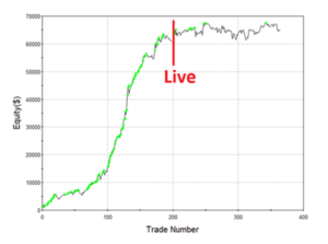
Curve-fitting is the fastest death for a trading or investment account once actual trading begins. Adding too many parameters and filters to improve your backtest feels good but rarely helps actual trading results in live markets.
Finding the perfect set of parameter settings to produce the perfect profit graph of past performance during strategy testing is a sure-fire way to curve fit and ultimately deplete your trading account.
Curve fitting is the black plague for system traders. The initial investment is often better donated than trading overfit strategies based on bloated hypothetical performance results.
In short, curve-fitting is finding patterns that are actually just random noise. As the curve fit trading strategy sees new data it will mistake random noise for predictive patterns causing trading losses. Preventing curve fitting and finding statistically significant patterns may be the key to your trading career
Why do Automated Trading Strategies Fail?

Most automated trading strategies fail due to curve fitting or overoptimization. There are numerous other factors, but overfitting and overoptimization are the prime suspects.
Beginning traders hunt for the holy grail strategy and get excited over “too good to be true” backtests or hypothetical trading results. Many think a profitable backtest means a license to print money and no financial risk.
Many say, “If I could find a set of rules or parameters that does well historically on a specific trading program then I will be set to achieve profits”. Unfortunately, the markets and trading do not work this way.
Too many algo traders focus on finding the perfect trading strategy based on hypothetical performance results with the highest profit instead of finding robust strategies that can withstand losses moving forward.
Robust strategies are ones that can withstand changes in market behavior and are not sensitive to small parameter changes (i.e., possess parameter stability). Additionally, robust strategies should pass a series of robustness tests that many traders are unaware of.
For those curious, I covered all these in detail here: Robustness Testing Trading Guide

Here are the 3 simplest ways to lower or avoid curve fitting risk

1. Out of Sample Testing

Out of Sample testing is simply withholding some data in your historical data set for further evaluation. For example, you have ten years of historical data and opt to put the last 30% in your back pocket.
You develop a great trading strategy on the first seven years of the data set – the in-sample data. You add filters, subtract rules, optimize parameters, etc. Once the strategy results are acceptable, whip out your “out of sample” data (the remaining 30% from your back pocket) and validate your findings.
If the strategy fails to produce similar results on the out of sample data, then you can be almost certain you have curve-fit to the first seven years of your data set.
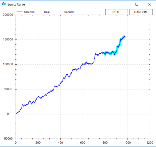
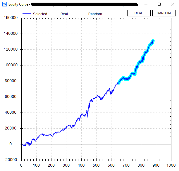
Below is a chart of an example strategy built using Build Alpha that highlights the out of sample period.
You like to see similar growth (and performance metrics) in both the in-sample and out-of-sample periods as sharp differences are often a red flag the hypothetical trading record was misleading.
On the other hand, successful OOS results are not necessarily indicative of future results and still involve financial risk but are a great first step to avoid overoptimization.
To read more about Out of Sample testing check out these blogs:

2. Sufficient Sample Size. Large number of trades

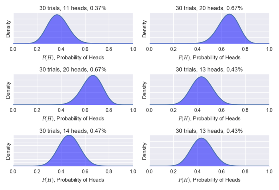
The second example of how we can reduce overfitting and hopefully our financial risk is to make sure your strategy has enough trades. If you flip a coin 10 times and it lands on heads seven times you cannot be certain you do or do not have a rigged coin.
However, if you flip a coin 10,000 times and it lands on heads 7,000 times then you can have high confidence it is a rigged coin.
Below is a photo of only 30 coin flips and below that is a photo of six different trials of 100,000 coin flips. You can see after a large number of flips things tend to converge toward the true expectation or their expected value. This is known as the Law of Large Numbers.
Trading Example

Let’s take this particular trading program below; it has a remarkably smooth cumulative profit graph and averaged $170 in profit per trade.
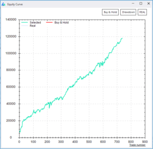
However, if we track this trading strategy’s average trade over time, we can see that in the beginning, when our trust in the trading system is lowest, it is a bumpy ride and far from the $170 per trade average. It takes about 100 trades for the average trade to converge to the actual results or average we expect!
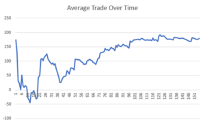
Most traders cannot stomach this short-term “randomness” and abandon ship. Traders that fall prey to strategy hopping never achieve profits and sadly never find out why. They never escape this short-term randomness.
My mentor explained this short-term randomness, long-term obviousness concept to me and a lightbulb clicked.
Escaping Randomness was the perfect title of my Chat with Traders interview where I discuss how to overcome trading randomness and why algorithmic trading can help traders think about markets and risk-taking in a more productive way. If you haven’t already, please check out Aaron’s wonderful work here: Escaping Randomness with David Bergstrom

3. Validate Across Other Markets

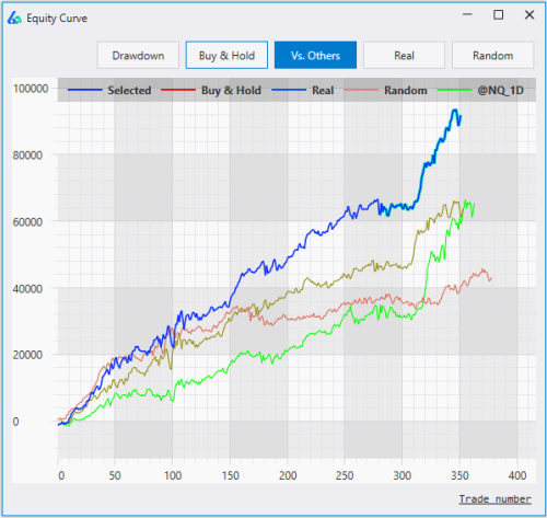
Test your trading system across other markets. If a particular trading program only works on one market, then it has a higher chance of being overfit than if a strategy performs profitably on a handful of markets.
I am not saying that a trading strategy that only works on one market is curve-fit – as there are many nuances, different players, and idiosyncrasies that exist within each market.
However, if a trading strategy performs across markets, then in such cases you can certainly have higher confidence that it less likely curve-fit than a strategy that only performs well on one data set.
Build Alpha Trading Strategies Across Markets Robustness Test
A sign of robustness is the ability to generalize to other data and withstand losses or is at least generally prepared for changes in the data.
Testing across similar markets is an easy way of quickly getting a sample of how well a strategy generalizes to new data sets.
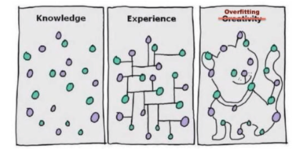
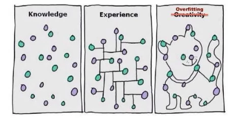
Think of the cat picture above. If we provide new data is this algorithm going to draw a dog? It is most likely not the next series of points. Testing on a new data set and not finding other animals would indicate that the cat was probably random.

Other methods to catch Curve Fitted Strategies before live trading

I cover most of these in the aforementioned Robust Trading Strategy Guide but here is a popular list for those eager traders looking for more than the three simplest material points to combat curve fitting risk.
These robustness checks identify curve fitting and overoptimization before the market does:

Vs Shifted

shift the start and stop time of each bar slightly. Re-trade the strategy on the shifted data sets. For example, hourly bars from 11:03 to 12:03 instead of 11:00 to 12:00.

Vs Noise

add and subtract random noise amounts to the market data. Re-trade the strategy on the noise adjusted time series

Vs Random

data mine for the best possible random strategy. Your strategy should beat this random benchmark if it contains true market edge

Monte Carlo Analysis

reshuffle and reorder the hypothetical trading results to see various paths the strategy could have taken. More on Monte Carlo Simulation here.

Variance Testing

resample from trade distribution only keeping strategies that have a performance metric some percent lower than the original backtest

Parameter Sensitivity Testing

trading systems that fail to show positive performance as parameters change are often curve fitted. For example, a moving average of 12 works but parameters of 11 and 13 result in substantial trading losses or losses similar to a random strategy.

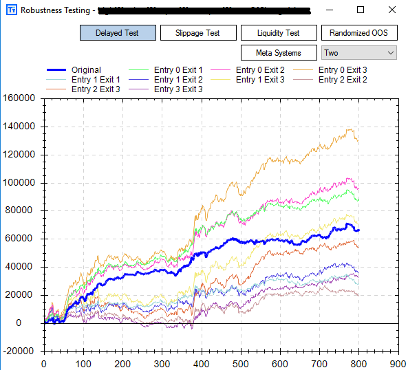
Delayed Testing

trading strategies that cannot perform similarly with slightly delayed entries or exits are potential substantial risk candidates

Liquidity Testing

trading strategies that are capacity constrained and cannot handle large amounts of capital are also potentially over fit models that will fail in live market trades

How can I reduce the risk of Curve Fit Strategies with Build Alpha

Build Alpha is professional algorithmic trading software that generates, tests and codes trading algorithms with no coding necessary. It is truly a no code algo trading software rich with features.
However, a large part of my research and testing over the past decade-plus of professional trading experience and software development has helped me develop and integrate these robustness tests into one piece of software – that is Build Alpha’s strength.
Build Alpha has all of the above listed tests available at the click of a button for use on any trading system it generates.
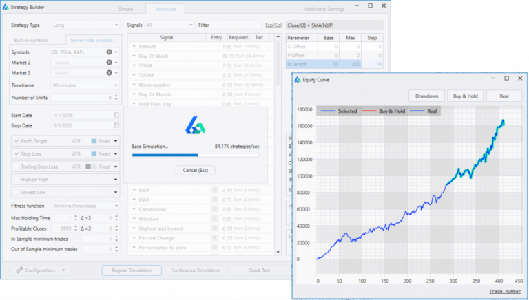
In plain English, there are many inherent limitations, and no amount of stress testing can completely account for curve fitting risk; however, as traders, all we can do is attempt to lower the probabilities that we have fit the data. Powerful software like Build Alpha exists to help traders easily test and validate trade ideas prior to exposing them to the market.

Many factors related, but avoiding overly optimistic hypothetical performance results, strategies with frequently sharp differences between testing periods, and highly sensitive parameter settings are good rules of thumb. However, it is important to use the robustness tests as much as possible as “eye-balling” has never been a solid approach to the markets.
Build Alpha comes complete with the litany of Robustness tests mentioned in this article. You can even import your own custom strategy to test inside Build Alpha.

How to avoid curve fitting in forex trading?

I get asked specifically about forex strategies and overfitting quite a bit. There are a few reasons I believe this to be a larger problem with forex trading than other asset classes.
First, forex has no central exchange, so fills are subject to the broker and essentially a function of his desires. Your historical simulated prices, backtest fills, and what happens in live can vary quite a bit.
Second, there are many forex scammers (I mean vendors) peddling overfit trading programs. The hypothetical performance results almost always differ from the actual results subsequently achieved in real markets. You can usually spot these guys by the too perfect equity curves and no knowledge of robustness testing.
This experience is not unique to forex markets but is certainly most prevalent here. There are other inherent limitations with buying trading systems, but this is not the place to discuss. It is best to build and test your own, so all risks are fully accounted for!

Curve Fit Key Takeaways

  • Past performance is not indicative of future results!
  • Curve fitting is a “too perfect” backtest that fails in actual trading
  • Curve fitting is the bane of most algo traders. Adversely affect trading results
  • Out of sample data is a first line of defense as it acts as unseen data
  • A large sample size of trades helps reduce the chances of finding something lucky
  • Validating across additional markets is a strong sign of robustness
  • There are more than three methods to help reduce the chances of curve fitting. Read more here: Robustness Testing Complete Guide

Three ways to reduce Curve Fit Risk Summarized

  1. Out of sample testing
  2. Require large sample size of trades
  3. Test across other markets

Summary

Algo traders constantly battle the market’s complexity with their own complexity often leading to curve fit or overfit strategies which cause substantial risk to actual trading results.
Overfit trading strategies are frail, too good to be true strategies that fail when the market changes or a particular trading program is exposed to new market data or market conditions.
Over optimizing parameters or memorizing material points of the historical time series are the common culprits of failed accounts. Is it avoidable?
Traders can use robustness tests and methods on trading systems to help reduce the chances of overfitting such as:
  • out of sample testing
  • ensuring a large enough trade count
  • testing their trading strategy on various different markets
These tests do not guarantee trading systems are not a fitted curve but function to help reduce the risk of curve fitting in the market. Build Alpha aims to make this identification and testing easy and with no coding necessary.
Thanks for reading,

Author

David Bergstrom – the guy behind Build Alpha. I have spent a decade-plus in the professional trading world working as a market maker and quantitative strategy developer at a high frequency trading firm with a Chicago Mercantile Exchange (CME) seat, consulting for Hedge Funds, Commodity Trading Advisors (CTAs), Family Offices and Registered Investment Advisors (RIAs). I am a self-taught programmer utilizing C++, C# and python with a statistics background specializing in data science, machine learning and trading strategy development. I have been featured on Chatwithtraders.com, Bettersystemtrader.com, Desiretotrade.com, Quantocracy, Traderlife.com, Seeitmarket.com, Benzinga, TradeStation, NinjaTrader and more. Most of my experience has led me to a series of repeatable processes to find, create, test and implement algorithmic trading ideas in a robust manner. Build Alpha is the culmination of this process from start to finish. Please reach out to me directly at any time.
Python Tips for Automated Trading

Python is the fastest growing and most popular programming language. This has drawn many quantitative traders, developers, and analysts to the easy-to-use and simple to understand scripting language. This post will cover a few python tips including reading text files, formatting dates and more essentials for automated trading.
Python has many popular finance and trading-based libraries for those that are interested in beginning their algo trading journey with python. The most popular trading library is probably talib which is a technical analysis library that has all the functions, indicators and math transforms an algo trader would need to start. Here is the talib documentation, if curious.
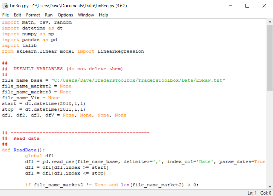
Reminder Build Alpha provides an easy way to get into automated trading without any programming. It does offer the ability to add custom signals via python for those of you that eventually want to learn or incorporate python into your process.

Is Python Good for algo trading

Python is an excellent choice for those traders that want to code themselves. The ease of learning, writing and understanding python code skyrockets it up the potential programming language list. Additionally, there are many good algo trading libraries that one can use freely. This saves the algo trader from having to recreate the wheel.
It is important to note that python does have its limitations when it comes to very large data sets or the need for speed. Other programming languages, like C++, are better suited for high frequency trading. I compare Python and C++ in my Algo Trading Guide.
The most popular python library, pandas, was created by a quantitative trading firm. AQR Capital Management began the project in 2008 before open sourcing it in 2009.

Why Python?

Python’s beauty is its simplicity. Python’s simplicity is its beauty. Unlike other programming languages, python does not use brackets to identify code blocks or semi-colons to end statements. Python simply relies on neatly written and indented code for the interpreter to grasp.
On top of the ease of use, Python’s mainstream popularity is due to the growing number of public libraries with python solutions. This gives many python coders an easy introduction to solving a problem or often a solution. For instance, no need to re-code a technical indicator if someone has already added it to the aforementioned talib library. You can simply access or use the code from talib.

Python Read in Financial Data

The first tutorial goes over how to read in a text file, format dates, and create new columns inside a pandas data frame. A data frame is a structure that stores your data in a convenient “table” for easy access. There are a few parts, but I will break down the code below.
The first thing we will do is import pandas library and call the built-in read_csv function. The read_csv function’s first input is the name of the file you desire to read in and store in your pandas’ data frame. The delimiter option allows you to specify the character that separates your text fields within your file.

import pandas as pd

df = pd.read_csv("ES.txt",delimiter=',')

Just like that, we have read a text file into a pandas’ data frame that we can now work with.
However, if we were to plot our data frame (closing prices) now the x-axis would simply be the number of bars as we did not specify an index column. In trading and time series analysis it is often nice to have dates as your x-axis.

Python Working with Dates

In the next few lines of code, I import a built-in python library that can read string dates (“12/30/2007”) and convert them into Python “DateTime” objects. To simplify this… we convert dates into Python dates.
I accomplish this by setting the built-in pandas index column to a list of newly Python formatted dates. I essentially loop through each string date, convert it, and add it to our data frame’s index. I then delete the original string Dates column.

from dateutil import parser

df.index = [parser.parse(d) for d in df['Date']]

del df['Date']

Now we can plot our closing prices and our x-axis will be dates.

df[‘Close’].plot()

To watch the video tutorial please head to YouTube: Python – Read in Text Files, Format Dates

Python Plotting Financial Data

In the code below I create a new column called “Range”. Notice how Python understands I want to do the calculation on all the highs and lows inside our data frame without me specifying so!
df['Range'] = df['High'] - df['Low']
Finally, the line below plots our Close and Range in two separate plots. This is from a previous tutorial video.
df[['Close','Range']].plot(subplots=True)

Python using the command line

The second part of this tutorial is to make our lives easier. Let’s say that we wanted to run that last program on a bunch of different stocks whenever we wanted. It would be quite annoying to open up the file or notebook and change the filename in our read_csv function every time.
Instead, we can create a filename variable and put the filename variable inside the read_csv function. Ideally, this filename variable could be dynamically set with user input from the command line.
This code is tricky and has a few moving parts. Below is the code and then I will explain what we did.

symbol = 'ES'

import sys,getopt

myopts,args = getopt.getopt(sys.argv[1:],"s")

for o,a in myopts:

        if o == '-s':

            symbol = str(a).upper()

            filename = "%s.csv" % symbol

            df  = pd.read_csv(filename,delimiter=',')

First, we created a symbol variable that will accept our user input. Second, we imported some built-in libraries and called the getopt function to read user input. We also specified that our desired input would be preceded by the “s” option.
We then wrote a simple for loop to read through all the command line inputs (which in this example is only one, but this template will allow you to create multiple command line input options). We then said, “if the command line option is ‘s’ then set the symbol variable to whatever follows it”. We also morphed “whatever follows it” into an upper case, string variable to avoid case-sensitive user input.
We then set our filename variable and proceeded to read our text file into our data frame (df) as before.
This is complicated, but a major time saver. Please review this video Python – Command Line Basics as the extra 3 minutes might save you hours of our life by utilizing tricks like this!

Python for Algo Trading with Build Alpha

Build Alpha is algorithmic trading software that creates thousands of systematic trading strategies with the click of the button. Everything is point and click and made for traders without any programming capabilities.
However, I recently added the ability to add custom entry or exit signals via python for those that want to get even more creative or have existing indicators they would want to throw into the Build Alpha engine.
This is the fastest road to algo trading with the most flexibility. It allows you to test without wasting time coding up every single idea, but still permitting you to add unique ideas via python whenever inspiration strikes. To see how you can add custom signals via python to Build Alpha please head here: buildalpha.com/python
This is complicated, but a major time saver. Please review the video as the extra 3 minutes might save you hours of our life by utilizing tricks like this!
Remember for those of you who don’t want to learn programming you can use research tools like Build Alpha to save even more time.
Thanks for reading,

Author

David Bergstrom – the guy behind Build Alpha. I have spent a decade-plus in the professional trading world working as a market maker and quantitative strategy developer at a high frequency trading firm with a Chicago Mercantile Exchange (CME) seat, consulting for Hedge Funds, Commodity Trading Advisors (CTAs), Family Offices and Registered Investment Advisors (RIAs). I am a self-taught programmer utilizing C++, C# and python with a statistics background specializing in data science, machine learning and trading strategy development. I have been featured on Chatwithtraders.com, Bettersystemtrader.com, Desiretotrade.com, Quantocracy, Traderlife.com, Seeitmarket.com, Benzinga, TradeStation, NinjaTrader and more. Most of my experience has led me to a series of repeatable processes to find, create, test and implement algorithmic trading ideas in a robust manner. Build Alpha is the culmination of this process from start to finish. Please reach out to me directly at any time.
Happy Friday!
For this Free Friday edition I want to talk about market regimes or market filters. I have a very simple intermarket filter or regime monitor to share.
The idea with market regimes or filters is to identify a condition or set of conditions that alters the market’s characteristics or risk profile. Ideally, you could find a bull and bear regime that would enable you to go long when in the bull regime and get into cash or go short when in the bear regime.
The simple regime filter I want to share was found using Build Alpha’s Intermarket signals. It only uses one rule and creates a clear bullish and bearish regime.
The rule says that if the Close of Emini S&P500 divided by the Close of the US 10 Yr Notes is less than or equal to the 10 days simple moving average of the Emini S&P500 divided by the 10 days simple moving average of the US 10 Yr Notes then we are in the bull regime.
Here it is in pseudo-code assuming eMini S&p500 is market 1 and US 10 Yr Note is market 2.
Bull = Close1/Close2 <= SMA(Market1,10) / SMA(Market2,10)
Bear=Close1/Close2  >    SMA(Market1,10) / SMA(Market2,10)
Let’s verify with some numbers that we have a discernible difference in market activity before I start flashing some charts at you.
Here are the S&P500’s descriptive statistics when in the bull regime:
  • Average Daily Return: 1.20
  • Std Dev Daily Return: 17.49
  • Annualized Information Rate:
1.09
Here are the S&P500’s descriptive statistics when in the bear regime:
  • Average Daily Return: -0.34
  • Std Dev Daily Return: 12.11
  • Annualized Information Rate:
-0.44
This would definitely qualify as something of interest. Let’s take a look at the equity curve going long when ES, the eMini S&P500 futures, enter into the bull regime.
It actually performed quite well with no other rules or adjustments only trading 1 contract since early 2002. It even looks to have started to go parabolic in the out of sample data (last 30% highlighted).
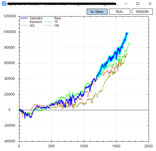
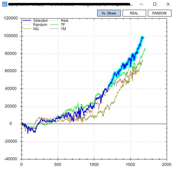
Build Alpha now offers another check for validity -> The ability to test strategy rules across other markets. This is very important when determining how well a rule generalizes to new (and different) data. The user can select whatever markets to compare against, but in the example below I chose the other US equity index futures contracts. You can see Nasdaq futures in gold, Russell Futures in green, and Dow Jones futures in red.
Now back to our Free Friday regime filter… Wouldn’t it be cool if the US 10 Yr Note performed well while Emini S&P500 was in the bear regime? That way instead of divesting from the S&P500 and going into cash we could invest in US 10 Yr Notes until our bull regime returned.
Well, guess what… the US 10 Yr Note Futures do perform better in the bear regime we’ve identified.
The best part is… Build Alpha now lets you test market regime switching strategies.
That is, invest in one market when the regime is good and invest in another market when the regime changes. This ability smoothed our overall equity curve and increased the profit by about 50%! Below is an equity curve going long Emini S&P500 in the bull regime and going long US 10 Yr Note Futures when the regime turns bearish.
Some major new additions coming to Build Alpha and I’ll be announcing them soon. As always thanks for taking the time to read these.
Happy Friday,
Old Posts:

Author

David Bergstrom – the guy behind Build Alpha. I have spent a decade-plus in the professional trading world working as a market maker and quantitative strategy developer at a high frequency trading firm with a Chicago Mercantile Exchange (CME) seat, consulting for Hedge Funds, Commodity Trading Advisors (CTAs), Family Offices and Registered Investment Advisors (RIAs). I am a self-taught programmer utilizing C++, C# and python with a statistics background specializing in data science, machine learning and trading strategy development. I have been featured on Chatwithtraders.com, Bettersystemtrader.com, Desiretotrade.com, Quantocracy, Traderlife.com, Seeitmarket.com, Benzinga, TradeStation, NinjaTrader and more. Most of my experience has led me to a series of repeatable processes to find, create, test and implement algorithmic trading ideas in a robust manner. Build Alpha is the culmination of this process from start to finish. Please reach out to me directly at any time.
Build Alpha’s Genetic Algorithm uses your inputs to create 1000s of trading strategies in seconds
Happy Friday!
For this Free Friday edition, I am going to do something new. I am going to make this slightly educational and give away some code.
I get tons of questions every week, but they mainly fall into two categories. The first question is in regards to adding custom data to Build Alpha. You can add intraday data, weekly data, custom bar type data, sentiment data, or even simple single stock data. The second question is in regards to using or learning Python.
In this post, I will attempt to “kill two birds with one stone” and show a simple Python code to download stock data from the Yahoo Finance API.
In fact, we will use Python to pull and save data ready formatted for Build Alpha for all 30 Dow stocks in less than 30 seconds.
You can view the entire script later in this code or in the video below.
The first few lines are simple to import statements pulling public code that we can reuse including the popular pandas library.
import pandas as pd
from datetime import datetime
from pandas_datareader import data
I then define a function that downloads the data using the built-in DataReader function of the pandas_datareader library. I also adjust the open, high, low and close prices by the split ratio at every bar. This ensures we have a consistent time series if a stock has undergone a split, for example. **Please note other checks could be recommended like verifying high > open and high > close and high > low, but I have left these up to Yahoo in this post**. I then end the function returning a pandas data frame that contains our downloaded data. This get_data function will be valuable later in the code.
def get_data(symbol, start_date, end_date):
dat = data.DataReader(symbol, "yahoo", start_date, end_date)
dat['Ratio'] = dat['Adj Close'] / dat['Close']
dat['Open']  = dat['Open']  * dat['Ratio']
dat['High']  = dat['High']  * dat['Ratio']
dat['Low']   = dat['Low']   * dat['Ratio']
dat['Close'] = dat['Close'] * dat['Ratio']
return dat
I then go ahead and put all 30 dow tickers in a Python list named DJIA. I also go ahead and create our start and end dates in which we desire to download data.
DJIA=["AAPL","AXP","BA","CAT","CSCO","CVX","KO","DD","XOM","GE","GS","HD","IBM","INTC","JNJ","JPM","MCD","MMM","MRK","MSFT",
"NKE","PFE","PG","TRV","UNH","UTX","V","VZ","WMT","DIS"]
start = datetime(2007,1,1)
end   = datetime.today()
Finally, and the guts of this code, I loop through all 30 of our tickers calling the get_data function on each one of them. After downloading the first one, AAPL in our case, I open a file named AAPL.csv and then loop through the downloaded price series retrieved from our get_data function. I then write each bar to the file appropriately named AAPL.csv. I then close the AAPL.csv file before downloading the second symbol, AXP in our case. This process is repeated for each and every symbol. The result is 30 seconds to download 30 stocks worth of data! Each symbol’s data is saved in a file named Symbol.csv.
for ticker in DJIA:
DF = get_data(ticker,start,end)
fh = open("%s.csv" % ticker,'w+')
for i,date in enumerate(DF.index):
fh.write("%s,%.2f,%.2f,%.2f,%.2f,%dn" % (date.strftime('%Y%m%d'),DF['Open'][i],DF['High'][i],DF['Low'][i],DF['Close'][i],DF['Volume'][i]))
fh.close()
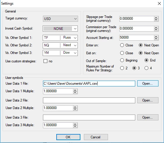
Now to the second part. Using this data in BuildAlpha is as simple as clicking on settings and searching for your desired file. I’ve attached a photo below that shows how the trader/money manager can now run tests on the newly downloaded AAPL data using the symbol “User Defined 1”. Pictures below for clarity.
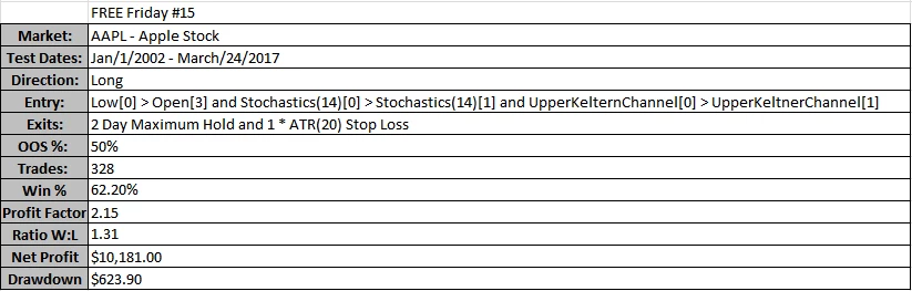
I’m showing a strategy created for $AAPL stock, but it is only to prove this Python code and Build Alpha feature work. There is major selection bias creating a strategy on a stock that has basically been in a major uptrend for 90%+ of its existence. That being said, and in a later post, I will show a new Build Alpha feature that allows you to test strategies across different symbols to make sure the strategy holds up on both correlated and uncorrelated securities. Either way here is the AAPL strategy.
Buy Rules:

1.Today’s Low > Open of 3 Day’s Ago
2.Today’s 14 Period Stochastics > Yesterday’s 14 Period Stochastic
3. Today’s Upper Keltner Channel > Yesterday’s Upper Keltner Channel

Exit Rules:

1. Two Day Maximum Hold
2. 1.00 * 20 Period ATR Stop Loss

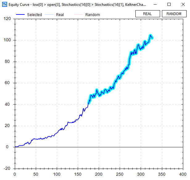
I like this strategy because it is convex. We limit the downside, but let the market give us as much as possible in 2 days. Below is the equity graph with the highlighted part being out of sample and based on 1 share as this is just for demonstration purposes!
I hope this makes life easier for some of you and as always… Happy Friday,
PS: This is all extra. You do not need to know Python (or any programming) to use BuildAlpha. This is just for advanced users that want additional help.
Old Posts:

Author

David Bergstrom – the guy behind Build Alpha. I have spent a decade-plus in the professional trading world working as a market maker and quantitative strategy developer at a high frequency trading firm with a Chicago Mercantile Exchange (CME) seat, consulting for Hedge Funds, Commodity Trading Advisors (CTAs), Family Offices and Registered Investment Advisors (RIAs). I am a self-taught programmer utilizing C++, C# and python with a statistics background specializing in data science, machine learning and trading strategy development. I have been featured on Chatwithtraders.com, Bettersystemtrader.com, Desiretotrade.com, Quantocracy, Traderlife.com, Seeitmarket.com, Benzinga, TradeStation, NinjaTrader and more. Most of my experience has led me to a series of repeatable processes to find, create, test and implement algorithmic trading ideas in a robust manner. Build Alpha is the culmination of this process from start to finish. Please reach out to me directly at any time.
What is Curve Fitting?

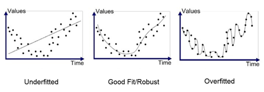
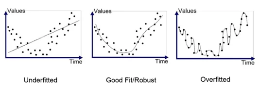
First, I need to describe over-fitting or more commonly known as curve-fitting. Curve-fitting is creating a model that too “perfectly” fits your sample data and will not generalize well on new unseen data. In trading, this can be thought of as your model too closely fits the historical data and will surely fail/struggle to adapt to new live data.

Here are two visuals I found to help illustrate this idea of curve-fitting.

How can we avoid curve fitting?

The simplest and best way to avoid (or reduce our risk of) curve-fitting is to use “Out of Sample” data. We simply designate a portion of our historical data (say the last 30% of the test period) to act as our unseen or “Out-of-Sample” data.
We then go about our normal process designing/testing/optimizing rules for trading or investing using only the first 70% of the test period or the “In-Sample” data.
After finding a satisfactory trading method we pull out our Out of Sample data and test on the last 30% of our test period.
It is often said that if the model performs similarly in both the in and out of sample data then we can have increased confidence the model generalizes well enough to new data.
No need to bring up selection bias or data mining here, but I will certainly cover it in another post/video series.

How can the human add value to the automated trading process?

The intelligent reader will question why we chose 30% and why the last portion of the data (as opposed to the first 27% or last 15%)?
The trader can add value and increase a trading model’s success by controlling the
  • Date Ranges of entire test
  • Out of sample location
  • Percentage of out of sample data

I have always heard that good science is often mostly attributable to good experimental design. In the trader’s case, good science would be setting up a proper test by choosing an appropriate test period, out of sample location, and out of sample percent.

Trading Data Example

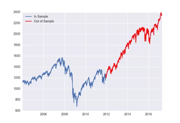
Let’s take a look at the S&P500 from 2004 to 2017. In the chart below I have designated the last 40% of the data to be our Out of Sample data.
This means we would create a trading model on the data from 2004 to roughly 2011 – the blue In Sample data. However, 2011 to present day (red Out of Sample) has been largely straight up.
If we build a long strategy that avoids most of 2008 via some rule or filter it may certainly do well in on our Out of Sample data simply because the underlying market went straight up!
You can see the importance of intelligently selecting your test period and out of sample period’s location and size.
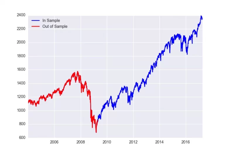
What if we used the first 40% of the data as our Out of Sample data? This provides a few benefits. First, it allows us to build our trading model on the most recent data or the last 60% of the data set – in our case 2009 to 2017.
Many traders will argue that they prefer to build their models on the most recent data as it is most likely the most similar to the live data they will soon experience. They then obviously test Out of Sample but just use older data and in our case 2004 to 2008 or the first 40%.
Now how did I know 40%? I simply looked at the chart and selected a percentage that would capture the financial crisis. My thought process is that if we train a model from 2009 to 2017 and then test it on 2004 to 2008 and it performs similarly in both periods then we surely have uncovered some persistent edge that generalizes over two unique sets of data. The two unique sets being our In-Sample (2009 to 2017) and our Out-of-Sample (2004 to 2008).
Selecting a proper location and percentage is mission critical. You want to design your test to be as difficult as possible to pass – try to break your system in the testing process. If you do not, then the market will surely break it once you start live trading!
Testing design and set up is undoubtedly where the human still adds value to the automated trading process. Build Alpha allows users to leverage computational power in system design, validation, and testing; however, the test set-up in BA is still an area where a smarter, more thoughtful trader can capture an edge over his competitors and add robustness to the output.

Bad Examples of OOS Data

Below I have some photos of some terrible experiment design to help drive the point home. Both present fairly simple out of sample tests to “pass”. Passing OOS testing is not the goal. Creating robust strategies is. This requires difficult OOS tests to pass (not what is pictured below). Please watch the video above for an explanation.

Takeaways

The main takeaway is that the human can still add value to the automated trading process by proper test/experiment design. That is why BuildAlpha software allows the trader/money manager to adjust everything (or nothing) from
  • Test Period
  • Out of Sample percent
  • Out of Sample location
  • In-Sample Minimum number of trades
  • Out of Sample minimum number of trades
I hope this was helpful – catch you in the next one,
For a more in-depth discussion check out

Author

David Bergstrom – the guy behind Build Alpha. I have spent a decade-plus in the professional trading world working as a market maker and quantitative strategy developer at a high frequency trading firm with a Chicago Mercantile Exchange (CME) seat, consulting for Hedge Funds, Commodity Trading Advisors (CTAs), Family Offices and Registered Investment Advisors (RIAs). I am a self-taught programmer utilizing C++, C# and python with a statistics background specializing in data science, machine learning and trading strategy development. I have been featured on Chatwithtraders.com, Bettersystemtrader.com, Desiretotrade.com, Quantocracy, Traderlife.com, Seeitmarket.com, Benzinga, TradeStation, NinjaTrader and more. Most of my experience has led me to a series of repeatable processes to find, create, test and implement algorithmic trading ideas in a robust manner. Build Alpha is the culmination of this process from start to finish. Please reach out to me directly at any time.
In this post I will go over a few different ways to manipulate price data to create visuals to aid in the investing and trading research process. I have attached a ten minute YouTube video that has explanations, etc. However, this post also attempts to briefly walk you through the Python code.
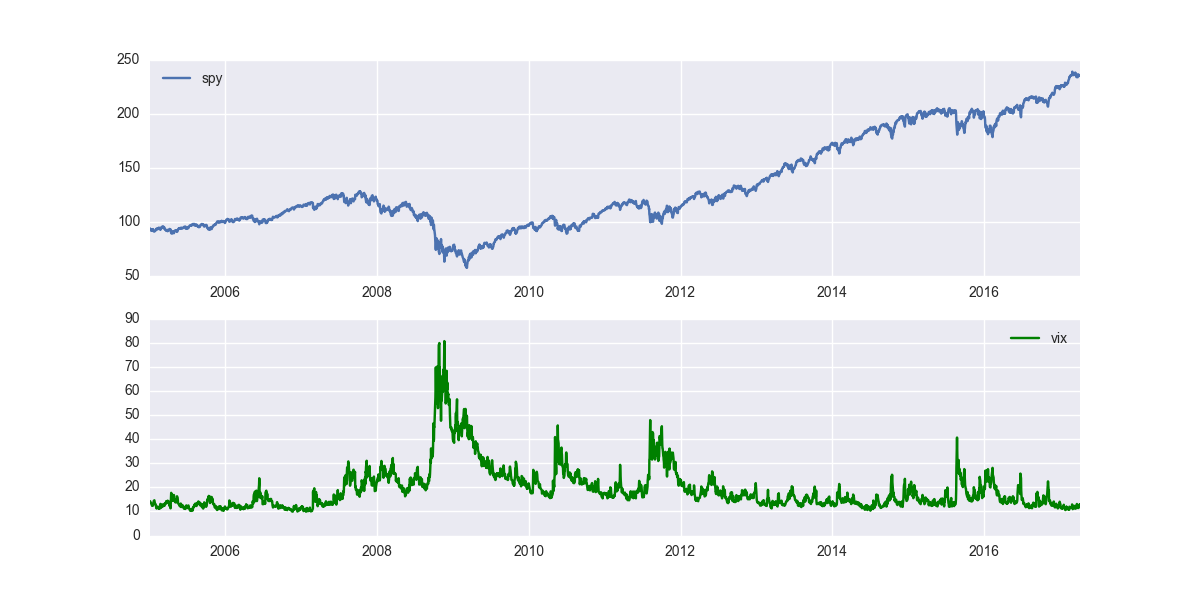
First, we will use some Python code to download some free data from the Yahoo Finance API. The code below creates a function called “get_data” that downloads and adjusts price data for a specified symbol over a specified period of time. I then download and store $SPY and $VIX data into a pandas dataframe.
import pandas as pd
import matplotlib.pyplot as plt
from datetime import datetime
from pandas_datareader import data
import seaborn as sns
print "Start Time: ", datetime.today().now()
def get_data(symbol, start_date, end_date):
dat = data.DataReader(symbol, "yahoo", start_date, end_date)
dat['Ratio'] = dat['Adj Close'] / dat['Close']
dat['Open'] = dat['Open'] * dat['Ratio']
dat['High'] = dat['High'] * dat['Ratio']
dat['Low'] = dat['Low'] * dat['Ratio']
dat['Close'] = dat['Close'] * dat['Ratio']
return dat
Ticker1 = get_data("SPY",datetime(2005,1,1),datetime.today())
Ticker2 = get_data("^VIX",datetime(2005,1,1),datetime.today())
df = pd.DataFrame(index=Ticker1.index)
df['spy'] = Ticker1['Close']
df['vix'] = Ticker2['Close']
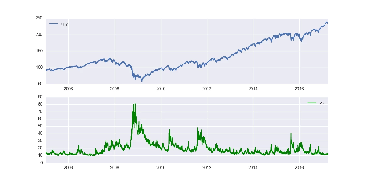
This next piece of code is two ways to accomplish the same thing – a graph of both SPY and VIX. Both will create the desired plots, but in later posts we will build on why it is important to know how to plot the same graph in two different ways.

1.
df[['spy','vix']].plot(subplots=True)

2.
fig, ax = plt.subplots(figsize=(12,6))
ax = plt.subplot(211)
plt.plot(df['spy'],label='spy')
plt.legend(loc=0)

ax = plt.subplot(212)
plt.plot(df['vix'],label='vix',color='g')
plt.legend(loc=0)
The first method is simple and straight forward. The second method creates a “figure” and “axis”. We then use plt.subplot to specify how many rows, columns, and which chart we are working with. For example, ax = plt.subplot(212) means we want to set our axis to our display that has 2 rows, 1 column, and we want to work with our 2nd graph. plt.subplot(743) would be 7 rows, 4 columns, and work with the 3rd graph (of 28). You can also use commas to specify like this plt.subplot(7,4,3).
Anyways, here is the output.
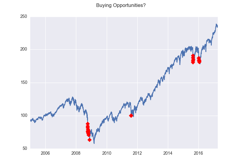
The next task is to mark these graphs whenever some significant event happens. In this example, I show code that marks each time SPY falls 10 points or more below its 20 period simple moving average. I then plot SPY and mark each occurrence with a red diamond. I also added a line of code that prints a title, “Buying Opportunities?”, on our chart.
df['MovAvg'] = Ticker1['Close'].rolling(20).mean()
markers = [idx for idx,close in enumerate(df['spy']) if df['MovAvg'][idx] - close &gt= 10]
plt.suptitle("Buying Opportunities?")
plt.plot(df['spy'],marker='D',markerfacecolor='r',markevery=markers)
This code creates a python list named markers. In this list we loop through our SPY data and if our condition is true (price is 10 or more points below the moving average) we store the bar number in our markers list. In the plot line we specify the shape of our marker as a diamond using ‘D’, give it the color red using ‘r’, and mark each point in our markers list using the markevery option. The output of this piece of the code is below.
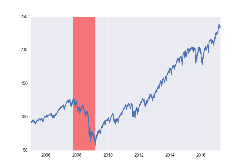
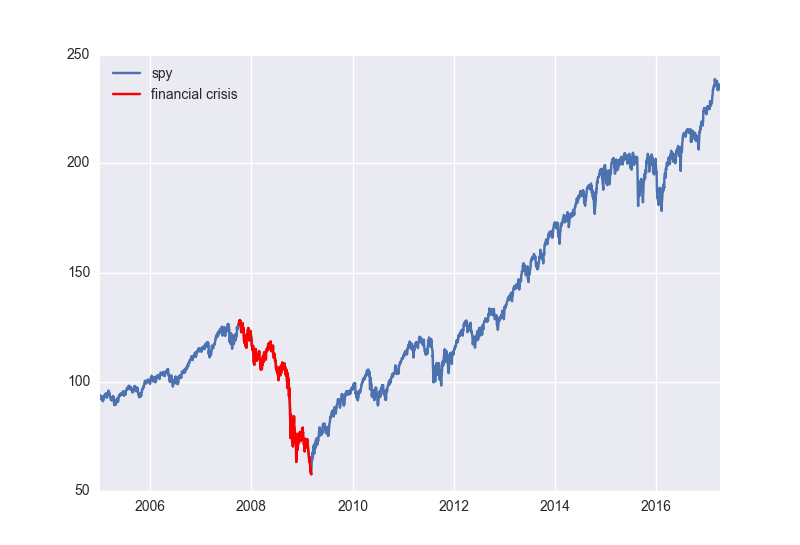
Next, and simply, I show some code on how to shade an area of the chart. This may be important if you are trying to specify different market regimes and want to visualize when one started or ended. In this example I use the financial crisis and arbitrarily defined it by the dates October 2007 to March 2009. The code below is extremely simple and we only introduce the axvspan function. It takes a start and stopping point of where shading should exist. The code and output are below.
fig, ax = plt.subplots()
ax.plot(df['spy'],label='spy')
ax.axvspan(datetime(2007,10,1), datetime(2009,3,9), alpha=0.5, color='red')
Personally I do not like the shading of graphs, but prefer the changing of the lines colors. There are a few ways to do this, but this is the simplest work around for this post. I create two empty lists for our x and y values named marked_dates and marked_prices. These will contain the points we want to plot with an alternate color. I then loop through the SPY data and say if date is within our financial crisis window then add the date to our x list and add the price to our y list. I do this with the code below.
marked_dates = []
marked_prices = []
for date,close in zip(df.index,df['spy']):
if date >= datetime(2007,10,1) and date <= datetime(2009,3,9):marked_dates.append(date)
marked_prices.append(close)
I then plot our original price series and then also plot our new x’s and y’s to overlap our original series. The new x’s and y’s are colored red whereas our original price series is plotted with default blue. The code and output is below.
fig,ax = plt.subplots()
ax.plot(df['spy'],label='spy')
ax.plot(marked_dates,marked_prices,color='r',label='financial crisis')
plt.legend(loc=0)
That’s it for this post, but I hope this info helps you in visualizing your data. Please let me know if you enjoy these Python tutorial type posts and I will keep doing them – I know there is a huge interest in Python due to its simplicity.
Also, I understand there may be simpler or more “pythonic” ways to accomplish some of these things. I am often writing this code with intentions of simplifying the code for mass understanding, unaware of the better ways, or attempting to build on these blocks in later posts.
Cheers,
Dave
It has been brought to my attention that Yahoo Finance has changed their API and this code will no longer work. However, we can simply change the get_data function to the code below to call from the Google Finance API
def get_data(symbol,start_date,end_date):
dat = data.DataReader(symbol,"google",start_date,end_date)
dat = dat.dropna()
return dat
Google adjusts their data so we do not have to. So I removed those lines. I also swapped out ‘yahoo’ for ‘google’ in the DataReader function parameters. Google’s data is also not as clean so I added a line to drop NaN values. That’s it. Simple adjustment to change data sources.
Thanks for reading,

Author

David Bergstrom – the guy behind Build Alpha. I have spent a decade-plus in the professional trading world working as a market maker and quantitative strategy developer at a high frequency trading firm with a Chicago Mercantile Exchange (CME) seat, consulting for Hedge Funds, Commodity Trading Advisors (CTAs), Family Offices and Registered Investment Advisors (RIAs). I am a self-taught programmer utilizing C++, C# and python with a statistics background specializing in data science, machine learning and trading strategy development. I have been featured on Chatwithtraders.com, Bettersystemtrader.com, Desiretotrade.com, Quantocracy, Traderlife.com, Seeitmarket.com, Benzinga, TradeStation, NinjaTrader and more. Most of my experience has led me to a series of repeatable processes to find, create, test and implement algorithmic trading ideas in a robust manner. Build Alpha is the culmination of this process from start to finish. Please reach out to me directly at any time.
Happy Friday!
For this Free Friday edition, I will just share an update of the Free Friday strategies performance.
One month is not indicative of anything and these are just meant for educational purposes (strategies may or may not have gone through the entire rigor of the robustness/validation techniques described on this site and offered within the software).
A lot of these strategies were built to demonstrate a specific Build Alpha feature and are for demonstrations purposes… always fun to track performance, however.
I post the strategies on Twitter and you can find them here: @dburgh or here: www.buildalpha.com/blog

Free Friday #1: Emini S&P500 -$312.50
Free Friday #2: Gold Futures +$600.00
Free Friday #5: Nasdaq Futures +265.00
Free Friday #6: Russell Futures +$1370.00, -$940.00, -$120.00, -$475.00, -$260, +$210.00, +$325.00, -$410.00, +$1050.00, +$185.00, -$1870.00, +$115.00, +$355.00, +$385.00
Free Friday #10: SMH Semiconductors ETF +$650.00
Free Friday #12: XLP Consumer Staples ETF +$100.00, -$180.00
Free Friday #14: GLD Gold ETF +$670.00

March Total: +$1,712.50
YTD Total: +$6,932.50
All in all, not a bad month. A few things to consider… 1. One month is by no means telling, but it is sure nice to see profits. 2. As mentioned not all these strategies went through the full spectrum of validation techniques. 3. Strategy #6 only has 1 rule so it is much more common for its entry condition to be satisfied; hence the larger number of trades each month. 4. All of these results based on 1 futures contract traded or 1000 ETF shares traded – very simple.
Please note I only include trades that are “live” or occur after I’ve publicly posted the strategy.
Also, the Free Friday strategies were by no means designed as a portfolio. Having a strategy, like FF6, trading frequently and others hardly trading at all would be ill-advised in most cases. These are simply for demonstration purposes and fun to track.
Happy Friday,
Old Posts:

Author

David Bergstrom – the guy behind Build Alpha. I have spent a decade-plus in the professional trading world working as a market maker and quantitative strategy developer at a high frequency trading firm with a Chicago Mercantile Exchange (CME) seat, consulting for Hedge Funds, Commodity Trading Advisors (CTAs), Family Offices and Registered Investment Advisors (RIAs). I am a self-taught programmer utilizing C++, C# and python with a statistics background specializing in data science, machine learning and trading strategy development. I have been featured on Chatwithtraders.com, Bettersystemtrader.com, Desiretotrade.com, Quantocracy, Traderlife.com, Seeitmarket.com, Benzinga, TradeStation, NinjaTrader and more. Most of my experience has led me to a series of repeatable processes to find, create, test and implement algorithmic trading ideas in a robust manner. Build Alpha is the culmination of this process from start to finish. Please reach out to me directly at any time.
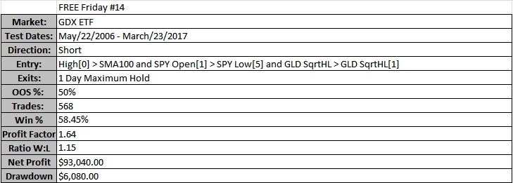
Happy Friday. The trader in me could not risk doing Free Friday #13 so I decided to release 2 strategies this week (14 and 14a).
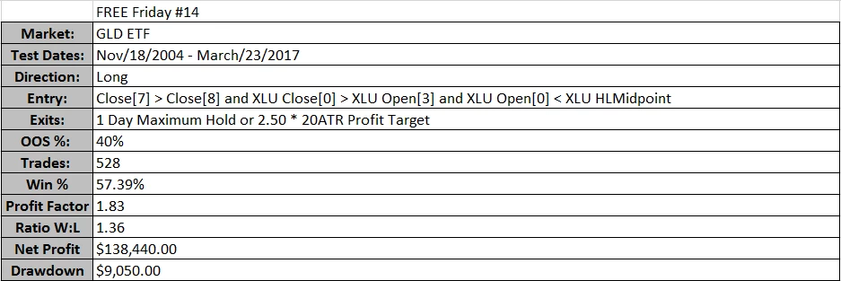
The first strategy shorts $GDX, the Gold Miners ETF, and the second strategy goes long $GLD, the Gold ETF.
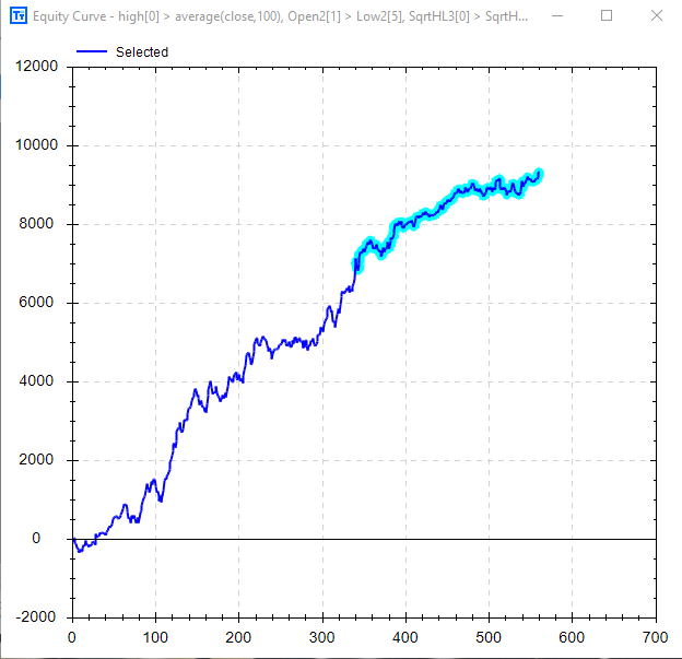
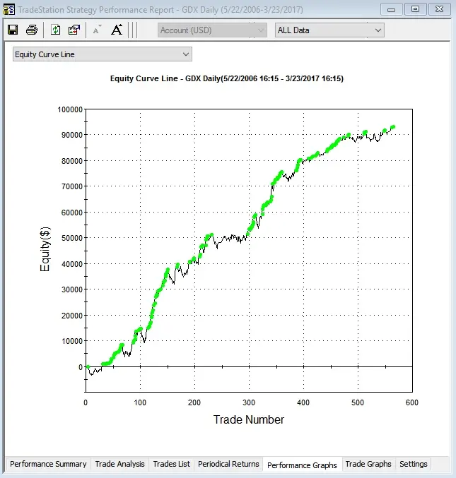
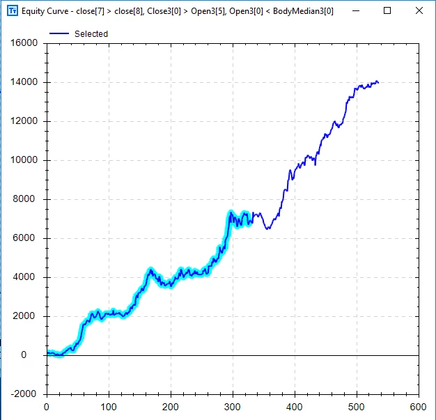
The strategy above is the GDX short strategy. The left chart is from Build Alpha (which now highlights out of sample trades – new feature) and the right chart is from TradeStation. Please note Build Alpha tested with only 100 shares per trade whereas the TradeStation charts in this post show results for 1,000 shares per trade. Below are the strategy results pulled from TradeStation.
Notice this GDX strategy takes Intermarket signals. One from SPY and one from GLD. The GLD signal is translated as the square root of this bar’s high * low is greater than the square root of the previous bar’s high * the previous bar’s low.
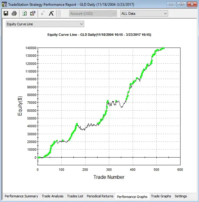
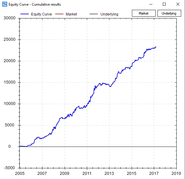
The second strategy is obviously the long GLD strategy. The chart below to the left is generated with Build Alpha using 100 shares per trade. The chart on the right replicated the strategy in TradeStation using 1,000 shares per trade (my laziness).
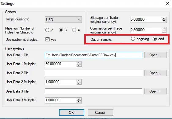
Please note the highlighted, out of sample, the section is at the beginning. Many traders prefer to build/train their model on the most recent data and use old data as the out of sample test data. Build Alpha now allows the trader this option through the updated settings menu (pictured later).
Please note the GLD strategy also uses Intermarket signals – in this case using XLU, the utilities ETF, for a pair of signals. Below I’ve attached a photo of the new settings menu to highlight how simple it is to change the out of sample period to the beginning or back to the end of the data.
Wrapping this up so you can get on with your weekend, I just want to show the combined chart of this long/short Gold strategy. Going Long GLD and short GDX when conditions are met. Obviously, and based on this post’s title, Build Alpha also permits multi-market portfolios now.
Happy Friday,
Old Posts:

Author

David Bergstrom – the guy behind Build Alpha. I have spent a decade-plus in the professional trading world working as a market maker and quantitative strategy developer at a high frequency trading firm with a Chicago Mercantile Exchange (CME) seat, consulting for Hedge Funds, Commodity Trading Advisors (CTAs), Family Offices and Registered Investment Advisors (RIAs). I am a self-taught programmer utilizing C++, C# and python with a statistics background specializing in data science, machine learning and trading strategy development. I have been featured on Chatwithtraders.com, Bettersystemtrader.com, Desiretotrade.com, Quantocracy, Traderlife.com, Seeitmarket.com, Benzinga, TradeStation, NinjaTrader and more. Most of my experience has led me to a series of repeatable processes to find, create, test and implement algorithmic trading ideas in a robust manner. Build Alpha is the culmination of this process from start to finish. Please reach out to me directly at any time.
Happy Friday. This week’s Free Friday strategy is for $XLP or the ETF that tracks US Consumer Staples. However, it was designed taking input from two other popular ETFs.
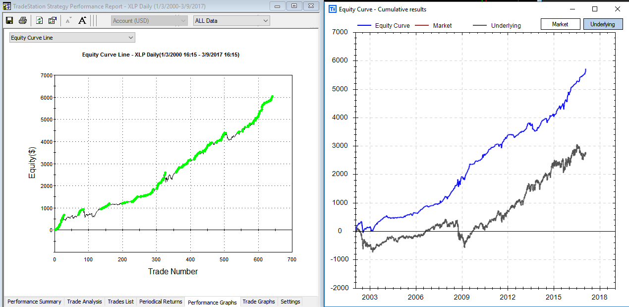
Here is the equity curve and backtest results. The left is a graph created by TradeStation and the right is a graph showing our backtest results (blue) and XLP buy and hold (grey). The chart on the right, created by Build Alpha, is plotted by date whereas the TradeStation chart is plotted by trade number – both software have the ability to plot both x-axis styles.
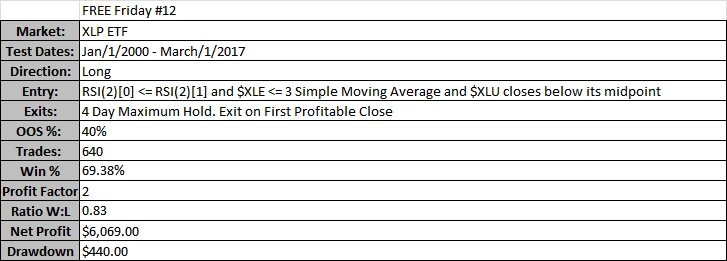
This strategy uses only 3 rules for entry
  1. XLP’s 2 Period RSI must be lower than it was 1 bar ago
  2. XLU – Utility ETF – must close below its midpoint
  3. XLE – Energy ETF – must be below its 3 period Simple Moving Average
The exits for this strategy are two-fold
  1. Maximum hold of 4 days
  2. Exit on the first profitable close
Below are the trade statistics for this Free Friday Strategy.
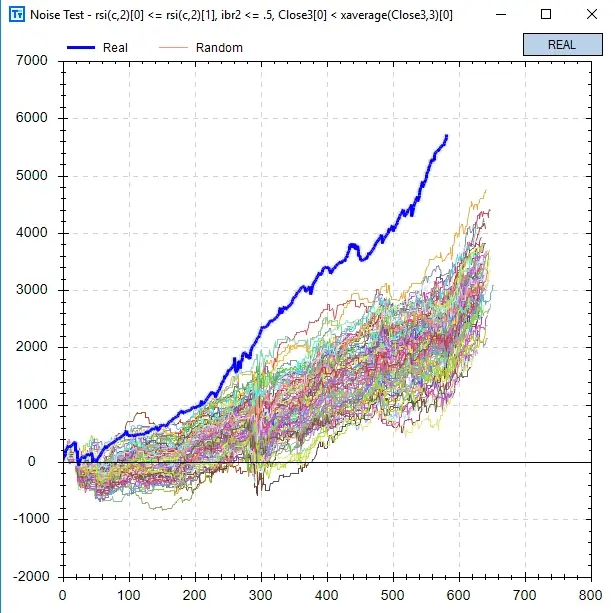
I know want to introduce another, and new, Build Alpha test to help validate trading strategies. I first mentioned this test here: Better System Trader Podcast. The Noise Test is a popular test that allows the user to randomly add AND subtract noise from the historical price data. The user can specify how much of the data he/she wants to adjust and by how much he/she wants to adjust the data.
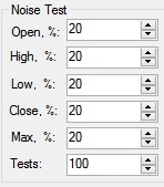
For example, the user can change 50% of the data by 25% of the average true range. This means we would adjust the data by either adding or subtracting up to 25% of the average true range to any of the opens, highs, lows or closes until we’ve adjusted 50% of the data.
We now have a “new” data set that contains a different amount of noise. Build Alpha will continue to create 100 new data sets all with differing noise characteristics. Finally, we will re-trade our strategy on these 100 new data sets to see how well it performs had the noise been different.
The idea is… does your strategy fall off a cliff if some other amount of noise is introduced or subtracted to your underlying data set?
I will show results for two noise tests I ran on this Free Friday strategy.
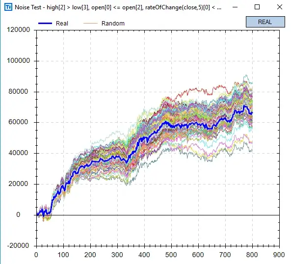
My first configuration was to adjust all the opens, highs, lows and closes at the same rate (20%). Furthermore, I only wanted to add or subtract up to 20% of the average true range whenever making a change.
As you can see the strategy is not very “anti-fragile”. That is, changing the noise amount never produced better results than our backtest. This can be a major red flag. However, the strategy still maintained general profitability over the 100 tests. I was pleased enough to run a second test. This time more creative with the adjustments to the data.
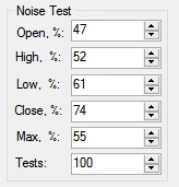
Adding or subtracting up to 55% of the average true range to differing amounts of the opens, highs, lows, and closes produced the above graph. This Noise Test has me much less confident in the strategy. For instance, our original backtest is now a significant outperformer. This generally means that it was too reliant to the underlying data. However, it does maintain overall profitability across the tests so may contain some actual edge nonetheless.
If up to me, I would continue researching this strategy and others as this is not an overwhelming pass.
The Noise Test is just another robustness check that Build Alpha offers to give traders and money managers every tool possible.
Happy Friday,
Old Posts:

Author

David Bergstrom – the guy behind Build Alpha. I have spent a decade-plus in the professional trading world working as a market maker and quantitative strategy developer at a high frequency trading firm with a Chicago Mercantile Exchange (CME) seat, consulting for Hedge Funds, Commodity Trading Advisors (CTAs), Family Offices and Registered Investment Advisors (RIAs). I am a self-taught programmer utilizing C++, C# and python with a statistics background specializing in data science, machine learning and trading strategy development. I have been featured on Chatwithtraders.com, Bettersystemtrader.com, Desiretotrade.com, Quantocracy, Traderlife.com, Seeitmarket.com, Benzinga, TradeStation, NinjaTrader and more. Most of my experience has led me to a series of repeatable processes to find, create, test and implement algorithmic trading ideas in a robust manner. Build Alpha is the culmination of this process from start to finish. Please reach out to me directly at any time.
What is an Equity Curve?

An equity curve is a plot showing the growth of capital over time from one specific trading strategy or portfolio. Said another way, an equity curve shows the cumulative profit of a trading strategy over time.
Algo traders look at equity curves as a first step in determining the viability of a trading strategy. For example, the equity curve below shows how an account would have performed had it traded only one contract using the fourth Free Friday strategy.
1b092c77-1215-48c5-8885-a58aae77178f
A rising equity curve warrants further investigation into a strategy’s robustness. Good strategies tend to move from the lower left to the upper right of the graph.
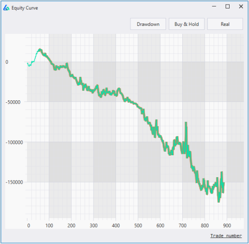
On the other hand, an equity curve with a negative return is moving in the opposite direction and most likely harmful for actual trading. A strategy like the one below can be discarded and does not need more of your time.
156fdde4-fca3-4f96-b547-55610bae6088

How to calculate an Equity Curve

To calculate an equity curve we simply add each successive trade to the rolling sum. Assume a trading strategy made the following five trades: +450, +200, -250, -200, +500. To calculate the equity curve, we would simply add the trade results after each trade.
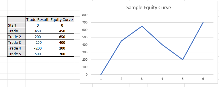
First, we have +450. Second, we have 450 + 200 or 650. Next, we have 650 – 250 or 400. Finishing this process results in the equity curve values +450, +650, +400, +200, +700.
What is Equity Curve Trading?

Equity curve trading, or managed equity curves, is using the equity curve of your trading strategy to make decisions about if you
  • should or should not take your strategy’s next trade
  • determine your next trade’s position size
  • should adjust your money management
A major fear in system trading is that often times your profit and loss or “equity curve” is your only feedback loop. That is, you don’t know when to stop trading a “broken” system until it has already cost you significant money.
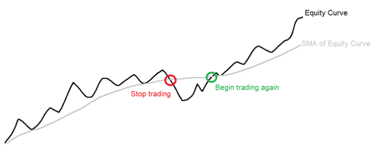
One industry idea is to monitor the equity curve in comparison to a moving average of the equity curve. That is, if our equity curve falls below its rolling average of the equity curve then maybe it is a red flag or early warning sign the system is broken. On the other hand, if you are confident in your system then maybe this temporary sign of system weakness is actually an opportunity to trade larger!
Below shows an example of applying this equity curve trading technique to your own strategy and using the moving averages of the equity curve to approve trading signals.
Some trading systems might miss significant drawdowns by simply turning off once the equity curve has weakened below its moving average and resume trading once the equity curve reclaims the moving average of the equity curve. The above example shows such.
Either way system traders need to know how their trading strategies perform when the equity curve weakens. If not, we are only to blame for our losses especially if we can identify some loss saving techniques ahead of taking a system live.

Equity Curve Trading Strategies

The trader should test various moving average parameter settings to find the best equity curve moving average to apply to each algo trading strategy. The most popular are the usual moving averages of lengths 5, 10 and 20 trades. Each strategy’s equity curve analysis will be different.
Most equity curve or performance-based systems can be defined as:
  • Skipping trades when equity curve is above a moving average of equity
  • Skipping trades when equity curve is below a moving average of equity
  • Skipping trades after consecutive winning trades
  • Skipping trades after consecutive losing trades
  • Skipping based on net profit
  • Skipping based on rolling Sharpe Ratio
Skipping or increasing size can be interchangeable. Optimizing moving average length or N trades for any of the above calculations can provide additional insights into improving trading strategies.
The autocorrelation of the trading strategy’s returns will determine if one should stop trading after the equity curve falls below its moving average or if one should increase size. If the strategy’s returns show strong negative autocorrelation, then the latter makes more sense.

Is my Strategy Working?

Many traders and small investors monitor raw equity curves to make a decision on a strategy’s health. If the strategy falls below its moving average does this mean the strategy is broken? A disciplined trader may be wise to evaluate the strategy once live trading net profit falls below the equity curve of the strategy.
However, wiser investment decisions based on strategy health and robustness are usually made using alternative stress tests. Equity curve strategies may reduce maximum drawdown but only where returns show serial correlation. That is, losses beget more losses and wins beget more wins.
For more on Strategy Health insights, please check out the Robustness Tests Strategy Guide.

Equity Curve Trading Software

Most brokerage platforms do not enable this type of functionality to execute equity curve trading. However, Build Alpha makes it simple to test any strategy for various equity curve trading strategies across all financial markets.

Build Alpha

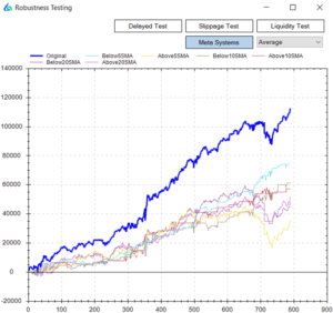
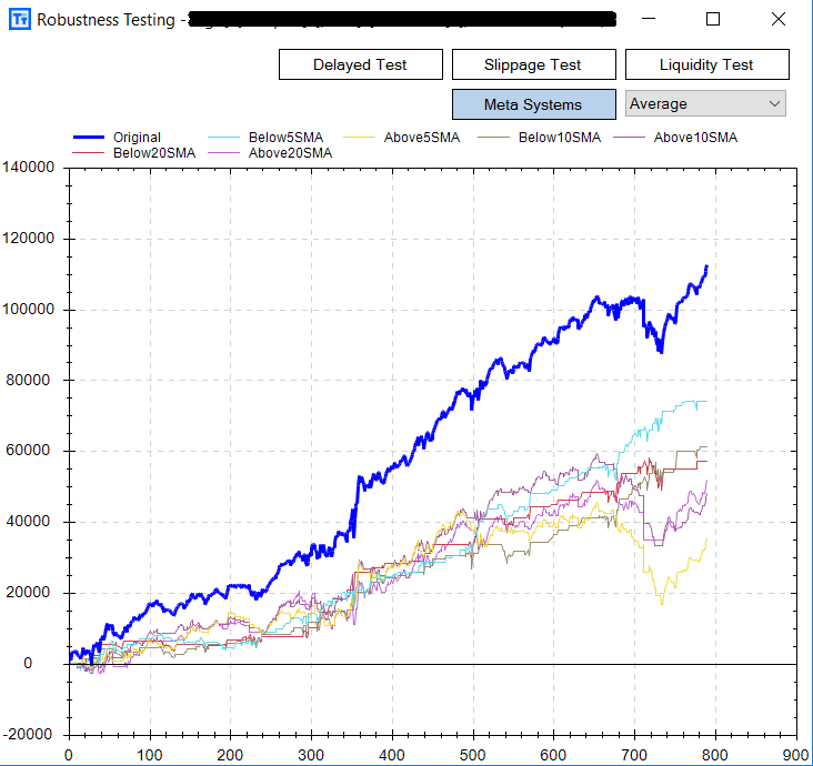
In the picture below you can see the thicker blue line represents our original backtest’s equity curve. This is how the strategy has performed ignoring all equity curve fluctuations. The nasty drawdown that concluded around trade number 740 is not a drawdown most traders could endure.
The baby blue line shows how the strategy performed only taking trades when the equity curve fell below its 5-period simple moving average. On the other hand, the yellow equity curve shows if you only took trades when the strategy’s equity curve was above its 5-period equity curve moving average.
You can see the baby blue returns are much smoother and avoided the most recent drawdown experienced around trade 740. In contrast, the yellow equity curve – only trading when the strategy was above its equity curve – caught all of the drawdown. In fact, the yellow equity curve had a worse drawdown than the original backtest.

Another Example

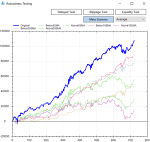
The blue and red lines show nice smooth returns whenever this strategy is below its 5 or 10 period equity curve moving average, respectively. On the flip side, the green and purple lines show how choppy and risky equity returns have been when only trading this strategy when above its 5 or 10 period equity curve moving average, respectively.

Need to Know

  • Equity Curve Trading can be applied to any asset class: stock market, futures, forex trading and even crypto currencies.
  • Equity Curve Trading can act as a money management technique and be applied to any used strategy.
  • The original strategy can use technical analysis, technical indicators, fundamental analysis, alternative data, data mining, various currency pairs, etc.
  • The most common equity curve trading strategy is comparing the cumulative profit of a trading strategy against a moving average of the cumulative profit. All things must be tested!
  • Build Alpha enables traders to monitor strategy results and numerous equity curve trading techniques.

Summary of Equity Curve Trading Strategy

Equity curve trading can provide valuable information that temporary weakness in a particular strategy has historically been followed by large drawdowns or by periods of out-performance and strategy recovery.
This knowledge can give insights to the trader on when to increase position size/leverage or to just simply have confidence in periods of equity curve drops, for example.
The main takeaway being… often smoother returns or a better risk-adjusted return can be achieved by considering the strategy’s “health” vis-a-vis the equity curve in relation to a moving average of the equity curve.
Following an equity curve trading technique will produce a new equity curve.

Update – Meta Strategies

Equity curve trading can be considered a Meta Strategy. A Meta strategy is a trading strategy that trades an underlying trading strategy. The idea is to develop an overlay strategy that will improve an existing trading system. Ideally, these layered decisions will increase overall net profit and performance as opposed to just following the original strategy.
The simplest Meta Strategy is to only take a trade if the underlying or original trading system’s last trade was a loser. Obviously, we can get more complex and say only trade if the original trading system’s last three trades were winners or, more probable, do NOT trade if the original trading system’s last three traders were winners.
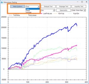
Build Alpha displays all the 2 and 3 trade meta strategy scenarios for each and every system. BA also shows equity curve trading results for every strategy.

Import Custom Strategies

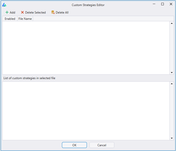
A key feature of Build Alpha is the ability to import trading systems built outside Build Alpha and run all the robustness and curve fitting tests on them. For example, you could easily import your systems, view their equity curves, and check all these meta systems on all of your trading systems. This is far more helpful than learning a new technical analysis technique.
The image above is Build Alpha’s custom strategy import window.
Thanks for reading,

Learn more about Build Alpha and Equity Curve Trading

Contact me for the demo and watch how Build Alpha can easily demonstrate the best equity curve trading strategies for any trading inputs.

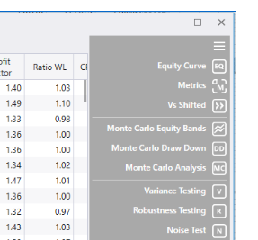
Locate the Robustness Testing Button

On the right-hand side of the results window, there is a button called ‘Robustness Testing’.

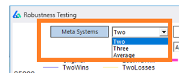
Change the Meta Systems view

Two displays all two trade scenarios such as: two consecutive wins, two consecutive losses, one win and one loss, one loss and one win, etc. Three displays all the three trade scenarios while Average displays moving averages of the equity curve trading.

Author

David Bergstrom – the guy behind Build Alpha. I have spent a decade-plus in the professional trading world working as a market maker and quantitative strategy developer at a high frequency trading firm with a Chicago Mercantile Exchange (CME) seat, consulting for Hedge Funds, Commodity Trading Advisors (CTAs), Family Offices and Registered Investment Advisors (RIAs). I am a self-taught programmer utilizing C++, C# and python with a statistics background specializing in data science, machine learning and trading strategy development. I have been featured on Chatwithtraders.com, Bettersystemtrader.com, Desiretotrade.com, Quantocracy, Traderlife.com, Seeitmarket.com, Benzinga, TradeStation, NinjaTrader and more. Most of my experience has led me to a series of repeatable processes to find, create, test and implement algorithmic trading ideas in a robust manner. Build Alpha is the culmination of this process from start to finish. Please reach out to me directly at any time.